Example of execution
In this notebook we reproduce the example presented in section 7 of the publication: Ll. Hurtado-Gil et al., Darkmix: Mixture Models for Detection and Characterization of Dark Matter Halos, submitted to ApJ
Used R packages and functions:
spatstatandspatstat.utils:owin,pp3,unique,as.im,quadscheme,box3,variablesinformulaandvolumeplotrix:draw.circleLaplacesDemon:BlocksandLaplacesDemonexpint:gammaandgammaincmisc3d:kde3dBase R: multiple functions (in particular the functionoptim)
Step 1 – Setup
Load the necessary functions and packages.
source("Code/darkmix.R")
library(spatstat)
library(spatstat.utils)
library(expint)
library(plotrix)
library(misc3d)
library(LaplacesDemon)
Read the data set to create the point process object and its quadrature:
data <- read.table("Data/datacat.txt")
minx <- 18; maxx <- 43;
miny <- 171; maxy <- 196;
minz <- 95; maxz <- 102;
clust <- pp3(x=data[,2],y=data[,3],z=data[,4], box3(xrange=c(minx,maxx), yrange=c(miny,maxy), zrange=c(minz,maxz)))
ntile <- c(50,50,14)
ntile <- c(100,100,28)
quad <- quad.3d(clust, ntile)
Declare a Finite Mixture Model of 10 cluster components plus background. Use Einasto profile for the clusters:
k <- 10
v <- 5
param2 <-c(k+1,rep(c(einasto.model,v),k), const.model,0)
Step 2 – Initial guess
Initialize the parameters vector and generate an initial guess of the cluster centers:
param <- rep(0,k*(v+1))
cent <- centers(clust, h=0.3, ntile=c(25,25,7), k)
arg <- list(centers=cent[[1]], re=1, n=3, mix=1, back=-2)
param <- mixture.model(param, param2, output=c(), action.initial, arg)
param_df <- param2profile(param)

##       x     y     z re n mix
## 1  33.5 178.5  99.5  1 3   0
## 2  36.5 192.5  98.5  1 3   1
## 3  39.5 174.5  97.5  1 3   1
## 4  25.5 189.5  98.5  1 3   1
## 5  20.5 192.5 100.5  1 3   1
## 6  38.5 193.5  96.5  1 3   1
## 7  37.5 175.5  99.5  1 3   1
## 8  33.5 172.5 100.5  1 3   1
## 9  32.5 185.5  99.5  1 3   1
## 10 21.5 190.5  98.5  1 3   1
## Background mix: -2
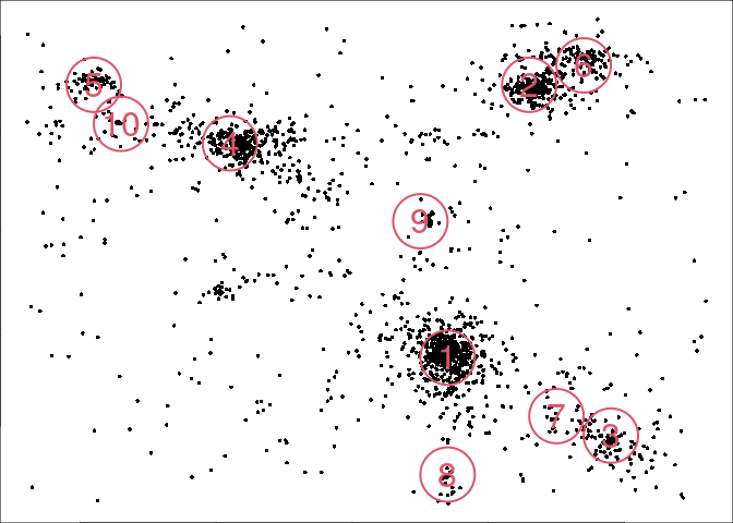
The initial guess can be visualized:
arg = list(mar=c(0,0,0,0), clust=clust, col=2, pch=16,border=2, cex=0.5, cexl=2, lwd=2)
out <- mixture.model(param, param2, output = NULL, action.draw, arg)
Step 3 – Likelihood maximization
Optimize the parameters via the Nelder-Mead algorithm, and save the result.
ocf <- optim(param, model.lik, param2=param2, model=mixture.model, clust=clust, quad=quad, all=FALSE);
param <- ocf$par
For further model refinement we can use the mask.freeze functions.
param <- mask.freeze(param, param2, mask.adjust_positions(k,v), clust, quad)
param <- mask.freeze(param, param2, mask.adjust_radii(k,v), clust, quad)
param <- mask.freeze(param, param2, mask.adjust_sersic(k,v), clust, quad)
param <- mask.freeze(param, param2, mask.adjust_mix(k,v), clust, quad)
The maximum likelihood, AIC and BIC can be calculated with
aic_bic <- AIC.BIC(param, param2, clust, quad)

## [1] "Maximum log-likelihood: 1348.04614787798"
## [1] "AIC: -2576.09229575595"
## [1] "BIC: -2237.65606617234"
However, the resulting parameters are still far from the best fit. Repeat the previous steps to obtain better results. In the following steps we present the results with the already obtained fit.
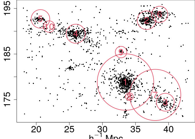
Visualize again to see the new model:
arg = list(mar=c(3,3,0,0), clust=clust, col=2, pch=16,border=2, cex=0.5, cexl=2, lwd=2)
out <- mixture.model(param, param2, output = NULL, action.draw,arg)
When the model is trusted, we can use it to estimate the number of particles per cluster:
arg <- list(clust=clust, quad=quad)
pop <- mixture.model(param,param2,output=c(), action.pop, arg)
pop

##  [1] 769.0515560 363.5435416 134.1685689 410.6648100  79.2871018 117.5140349
##  [7]  20.9611194   0.8541122  35.9582149  15.8071338 133.1898065
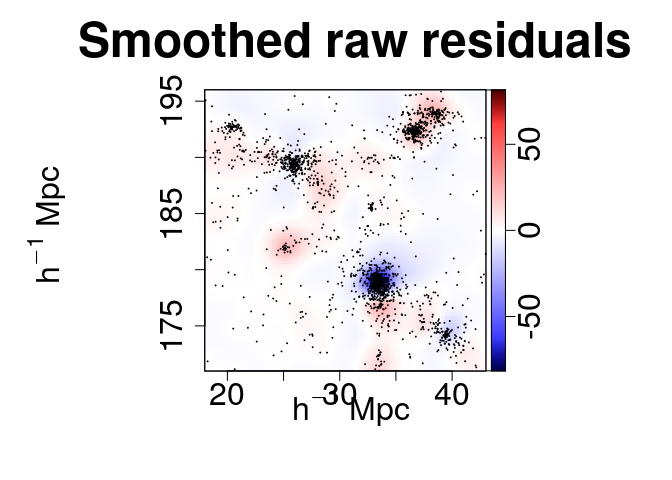
Step 4 – Goodness of fit
The goodness of fit can be evaluated with the function goodness
(calculation might take several minutes).
goodness(param, param2, clust, quad, ntile, residual.type="raw", bandwidth=1)

## [1] 0.9254999
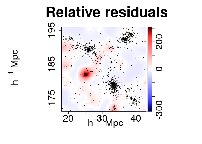
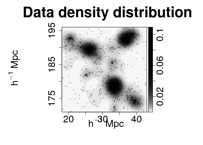
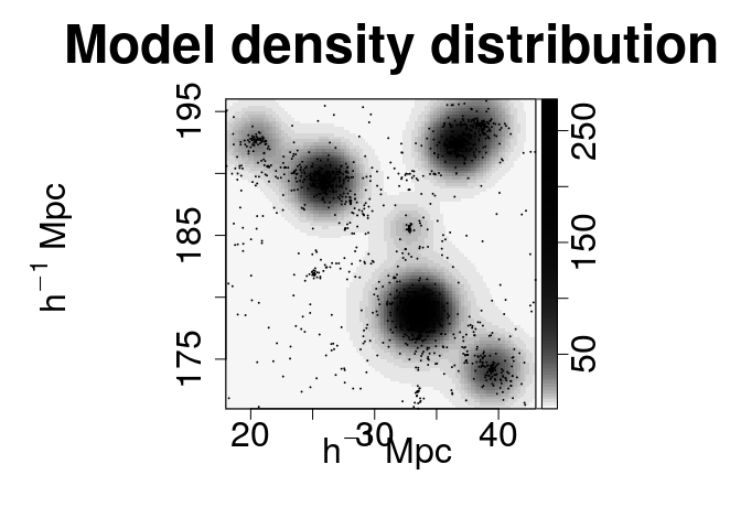
The different kernel density fields can be generated at once. By order of appearance: absolute residuals, relative residuals, data density field and model density field.
maps <- c("s", "e", "d", "m")
plot.mm3d(param, param2, clust, quad, residual.type="raw", bandwidth=1, maps=maps, fast=TRUE, col.point=1, scale="log", proj.var="Z", print=FALSE, print.data=TRUE, w=880, h=880, ntile=ntile)
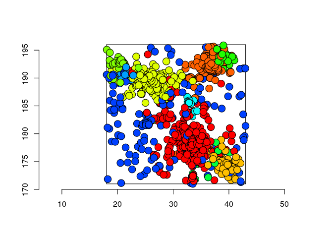
The membership of each particle to the clusters can be obtained and plotted as follows:
classification <- membership(param, param2, mixture.model, clust, threshold=0.3, print=FALSE)
Another possibility is to generate new samples reproducing the original data set (if a component has very few particles warnings might appear).
window <- clust$domain
num_particles <- data.frame(table(classification[[1]]$class))
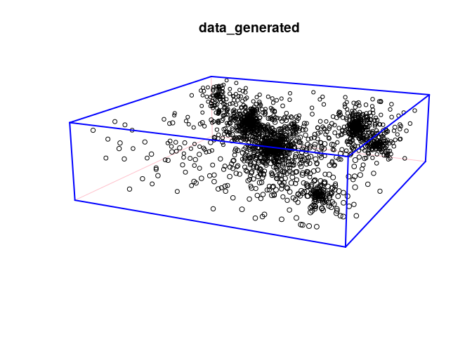
data_generated <- gen.pattern(param, param2, num_particles, window, scl=4)
Visualize the new sample with
plot(data_generated)
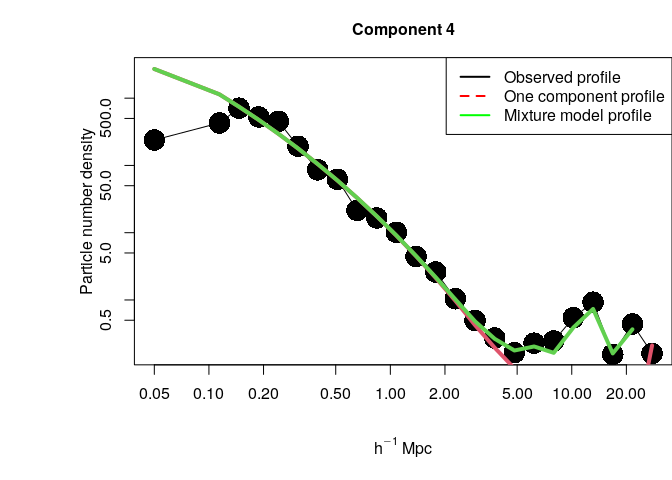
We can visualize as well the empirical density profile centered in a given component together with the full model and the single component estimations. For example, for component 4:
comp <- 4
profiles <- plot.profile(param, param2, clust, comp, xlim=c(0.1,40), nbin=25, flag.legend=TRUE)

## Warning in cbind(emp.pro, comp.pro[, 2], mm.pro[, 2]): number of rows of result
## is not a multiple of vector length (arg 3)